Maximizing Basketball Training Volume and Efficiency

")


")

Back in my youth basketball days, my coach used to yell, “Only one stat matters: who scored the most points!” That mindset—focused purely on raw output—ignored the deeper layers of what drives success on the court. Today, as basketball analytics evolve, it’s clear that volume (how many shots you take) and efficiency (how well you convert them) are the twin pillars of performance.
This article breaks down how these two core metrics offer coaches a powerful framework for understanding and improving team performance—at any level of the game.
You can follow me on Twitter
“ONLY ONE STAT MATTERS: WHO SCORED THE MOST POINTS”
I don’t think I’m taking much of a risk by saying that the author of these words – my coach back in my youth basketball days – probably isn’t someone who pays for an annual subscription to Cleaning The Glass. For him, the only stats we had access to at our level – namely, the total number of points scored by each player – weren’t just useless; they were downright harmful to our collective goal, which was constantly undermined by our obsession with shining individually (the way some of us would sprint toward the stat sheet the moment the final buzzer sounded suggests he wasn’t entirely wrong).
As for me, I gradually developed a taste for analytics (the collection, analysis, visualization, and interpretation of statistical data) as I digged deeper into the game, particularly through the lens of the NBA. However, I stayed skeptical for quite a while about actually using data in my own coaching work, mainly for two reasons:
1° Designing a method to collect reliable data for analysis seemed too challenging logistically speaking
2° The multitude of statistical concepts I was studying, although extremely insightful, appeared far too sophisticated to serve as relevant analysis tools at an amateur level
Over the past few months, I’ve gradually reconsidered my stance, thinking back to that old saying. Like many of the classic catchphrases coaches like to use, it’s something of a truism: after all, the ultimate goal of a basketball game is indeed to score more points than your opponent. Fair enough. But once you’ve stated that, can you really argue that the ever-growing pool of statistics produced in professional basketball offers no added value when you’re in charge of a team ? Is there truly no data that could help guide our work toward optimizing performance ?
Starting from the opposite assumption, and before worrying about how I would practically go about producing the statistical indicators I would need, I began by asking myself a basic question: what are the essential pieces of information a coach needs to assess a team’s performance, regardless of the level they’re playing at ? This process of prioritization led me to study the nature of the game itself, in an effort to identify fundamental trends that could be evaluated statistically. As I dove deeper into my research and reflection, my perspective on basketball evolved: I came to see a game as the sum of two essential battles – one to dominate shot volume, and the other to dominate shooting efficiency. These two pillars of basketball performance, along with the methods for assessing them, will be the focus of this article.
“THE TWO SIDES OF BASKETBALL”
The dichotomy I’m proposing is probably not the most intuitive, even for someone familiar with basketball. There’s actually a much more obvious, more universal one that applies to all invasion sports, and one that’s far more common when analyzing a team’s results: the division between offense and defense. This remains absolutely essential for understanding the game for a variety of reasons, including the fact that its temporal and spatial boundaries are crystal clear to anyone watching a game or playing the sport. Additionally, there’s a general consensus on how to effectively evaluate a basketball team’s performance in both areas: offensive rating and defensive rating.
These two indicators present several major advantages:
1° The ability to measure a team’s overall performance level on both offense and defense with a single numerical value
2° The ability to measure a team’s performance relative to others based on a common reference point: possession (a concept we’ll revisit later). This allows for fair comparisons between the performance levels of competing teams
3° And finally, the fact that they are mirror indicators, calculated in the same way, so they can be combined to produce a single metric evaluating a team’s overall performance: the net rating, which is calculated as offensive rating – defensive rating.

The graph produced from these statistical indicators for the 2024/2025 NBA season clearly visualizes the performance level of each team in both offensive and defensive areas. The overall performance level, quantified by the net rating number displayed next to each team’s logo, is also easily perceptible: the closer a team is to the top-right corner of the graph, the better its overall performance, and vice versa. From this data, several key insights can already be drawn. Among the most obvious: the Celtics, Cavaliers, and especially the Thunder have reached performance levels far above the other teams; the Magic has one of the best defensive teams in the NBA but struggles significantly on the offensive end, unlike the Suns, …
As a coach, offensive rating and defensive rating appear to me as valuable indicators for a general evaluation of my team’s performance. However, at the level I operate at, they seem to be somewhat disconnected from my actual needs, for one main reason: these indicators provide a “what”, that is, an evaluative measure of performance, but they don’t give any insight into the “how” or “why” behind those offensive and defensive performances. While additional video analysis can help me identify some clues, other statistical indicators might help me more precisely pinpoint specific strengths or weaknesses to focus my coaching efforts on.
THE POSSESSION REFERENCE FRAME
Anyone who regularly consults websites like the NBA’s or Basketball Reference has likely noticed the abundance of various statistics that professional leagues and specialized sites are now able to produce, especially thanks to new technologies developed, for example, by Second Spectrum. Twitter and YouTube are now flooded with accounts and channels producing basketball content that is at least partially based on analytics. As a coach, however, this wealth of information raises the necessary question of how to prioritize the data. Is there a way to discriminate these indicators based on their importance in evaluating the “how” and “why” of a team’s overall performance ? A ranking criterion between “primary” data and “secondary” data that would allow coaches with limited resources to focus on the former ? To answer these questions, let’s try to approach a basketball game from a similarly primary perspective.
A basketball game is an entity that breaks down into a series of back-and-forth possessions on each side of the court. At the end of each possession period, the opposing team takes possession of the ball, and this continuous alternation of possessions between the two teams dictates the pace of the game (with each team’s period of ball control limited by a clock) and ensures a near-equivalence in the number of possessions played by both teams over the course of a game (end-of-quarter possessions can slightly favor one team). This equivalence explains why the concept of possession is used as a reference point for calculating ratings: these indicators can estimate, with an equal number of possessions (conventionally normalized to 100), a team’s ability to score and defend points across several games without being biased by “statistical inflation” from a game played at a breakneck pace, for example.
Adopting this perspective, a basketball game becomes a battle for better maximizing the value of possessions compared to the opponent, meaning both the effort to ensure our offensive possessions result in as many points as possible, and to make our defensive possessions lead to as few points conceded as possible. The team that wins the duel will thus be the team that has made the best use of the nearly equal number of possession phases that both teams have had.
How can we evaluate, beyond the simple rating obtained, the “how” and “why” of the success or failure of a possession ? By starting with determining its possible outcomes.
THE FOUR FACTORS
Upon further reflection, the outcome of a team’s possession period can only take a limited number of configurations, more or less favorable. There are three possible outcomes:
1 – The team takes a field shot, which either goes in the basket or is grabbed by an opposing player (through a defensive rebound or out-of-bounds play) → the opposing team regains possession of the ball
2 – The opponent commits a foul that sends the team to the free-throw line, and the series of free throws ends either with a made free throw or with the ball in the hands of an opposing player → the opposing team regains possession of the ball
3 – The team loses the ball due to an interception, out-of-bounds play, a rule violation, or the shot clock violation → the opposing team regains possession of the ball
However, if the team takes and misses a shot (a field shot or on the final free throw of a serie) and the ball ends up in the hands of one of their own players (through an offensive rebound or a loose ball recovered by the offense after a missed defensive rebound), they retain possession until one of the three previous scenarios occurs.
Given this observation, we can logically calculate the number of possessions played by a team in a game using the following formula: FGA (field goals attempted) + {FTA*0.44} (estimated number of series of free throws1) + TOV (turnovers) – ORB (offensive rebounds).
To the 4 parameters in this formula, which at this stage are raw volumes, we can thus associate indicators that assess the team’s performance in these specific areas:
1 – The effective field goal percentage (or eFG%), which measures shooting efficiency, taking into account the added value of three-point shots
→ The higher the number, the more effectively the team is using its possessions when they manage to take a field shot
Example: In 2024/2025, the Cavaliers scored an average of 57,8% of their field goal attempts (accounting for the value of a three-pointer), while only allowing 52,8% of their opponent’s field goals. This represents an average of 0,1 points per field goal more than their opponents
2 – The turnover percentage (or TOV%), which measures the ratio of turnovers per 100 possessions
→ The lower the number, the more effectively the team is using its possessions by limiting the proportion that ends without a shot attempt
Example: In 2024/2025, the Thunder forced their opponents to turn the ball over on 14,9% of their possessions, while only turning the ball over themselves on 10,3% of their possessions. This represents, for every 100 possessions played, an average of 4,7 fewer possessions without any shot attempts for the Thunder compared to their opponents
3 – The offensive rebound percentage (or ORB%), which measures the ratio of offensive rebounds grabbed during situations with a chance to secure an offensive rebound (missed field goal or missed last free throw of a serie)
→ The higher the number, the more effectively the team is using its possessions by increasing the proportion in which it gains an additional shot opportunity
Example: In 2024/2025, the Rockets grabbed an offensive rebound on 31,7% of their missed shots, while only allowing their opponents to grab offensive rebounds on 23,8% of their missed shots. This represents, for every 100 possessions played, an average of 7,9 more second-chance opportunities for the Rockets compared to their opponents
4 – The free throw rate (or FT Rate), which measures the ratio of free throws made to field goals attempted
→ The higher the number, the more effectively the team is likely using its possessions by increasing the proportion where they get to the free throw line (assuming that free throw success is – except in rare cases – higher than field goal success)
Example: In 2024/2025, the Lakers made an average of 21,3 free throws for every 100 field goal attempts, while allowing their opponents to make only 17,8 free throws for every 100 field goal attempts. This represents, for every 100 field goal attempts, 3,5 more free throws made by the Lakers compared to their opponents
These indicators, first introduced by analyst Dean Oliver in his book Basketball on Paper and known as the Four Factors, are considered “primary indicators” in the sense that, with these 8 factors (4 for offense, 4 for defense), we can maintain an overview of the quality of possession management by the team while delving into the specific causes. These tools are extremely valuable for a coach because they allow for a concrete evaluation of the effects of any changes made, regardless of their nature. In fact, the mission of every team and its coaching staff, whether they are aware of it or not, is essentially to make decisions that positively impact at least one of these 8 factors without negatively affecting the others proportionally.
THE OTHER DICHOTOMY
This concentration of performance evaluation within 4 unique factors, when stated by Dean Oliver following the release of his book in 2004, represented a major evolution for professional team staff. However, upon closer inspection, it seems possible to propose an even more synthetic approach based on these elements. Indeed, by digging deeper into the reflection on these factors, we can observe that each of them actually measures really 2 distinct differentials:
1 – The differential in shot volume, meaning the ability of a team to take more shots (whether in play or via free throws) than their opponent given the same number of possessions
2 – The differential in shooting efficiency, meaning the ability of a team to score more points than their opponent given the same number of shots (whether in play or via free throws)
Viewed from this angle, a basketball game can only be won if our team has at least one positive differential in both areas, and if the differential in our favor is decisive enough to cover any potential deficit recorded in the other area. Thus:
1 – If we assume that a possession should typically corresponds to a shot attempt, the ability to grab more offensive rebounds than the opponent (ORB%) on one hand, and the ability to commit fewer turnovers than the opponent (TOV%) on the other, both contribute to the same phenomenon: increasing the difference in the average number of shots attempted per possession by our team compared to that of our opponent
→ It is possible to more simply calculate the shot volume differential per possession between two teams using the following formula: (FGA – opponent’s FGA) / 100 possessions
2 – The ability to score at a higher effective shooting percentage than the opponent (eFG%) contributes to increasing the difference in the average number of points scored per shot attempt by our team compared to that of our opponent
→ It is also possible to calculate the shooting efficiency differential between two teams using the following formula: eFG% – opponent’s eFG%
The graphical representation of these two differentials gives us the following result:

Unlike the previous graph, this one no longer provides information about the performance disparities a team may have between the offensive and defensive phases; however, it does give much more insight into the playing style of the teams involved. For example, we can see that the Celtics and the Cavaliers mostly rely on a positive shooting efficiency differential to boost their net rating, while the Warriors and the Rockets focus more on a higher volume of shots than their opponents to do so. The Thunder, on the other hand, manages to dominate the NBA in both volume and overall efficiency.
The most attentive will have noticed that one of the 4 factors has not been accounted for in the calculation of efficiency and volume. This fourth factor actually has the particularity, due to the way its formula is structured, of combining the evaluation of both volume and efficiency at the free-throw line into a single indicator, the FT Rate. However, it is possible to separate these two elements in order to measure them individually:
→ The free throw percentage (FT%), the free throw success rate, for which we can calculate the differential using the formula: FT% – FT% of the opponent, can be merged with the field goal percentage into a global shooting success indicator, the true shooting percentage (TS%), thus allowing us to obtain the overall shooting success differential using the formula: TS% – TS% of the opponent
→ The free throw attempts percentage (FTA%), the ratio of free throw attempts per 100 possessions, for which we can calculate the differential using the formula: ({FTA*0.44} – {FTA of the opponent*0,44}) / 100 possessions, can be merged with the field goal attempts per 100 possessions into a global shooting volume indicator, the total shot attempts (TSA), thus allowing us to obtain the shot volume differential per 100 possessions using the formula: TSA – TSA of the opponent
The graphing of these two newly adjusted indicators gives the following result:

While the results obtained through these two indicators are necessarily more accurate since they incorporate all possible scenarios for the outcome of a possession, I personally don’t think they are necessarily more relevant than the previous one as an analysis tool for the coach:
1° On one hand, in terms of volume assessment: the coach, and by extension the team, seem to have only a partial influence on the number of free throws called for both sides. While certain strategies (notably the hack) can significantly increase the free throw attempts ratio, this ratio seems relatively dependent on a contingent factor for the coaching staff, namely how the games are officiated
2° On the other hand, in terms of efficiency assessment: the coach, and by extension the team, also has an extremely limited margin of maneuver over the general free throw success rate (other than by creating a rotation of reliable shooters), as these shots are, by definition, undefended. Again, the hack seems to be the only lever available for the coach to alter the opponent’s free throw percentage.
THE PRIMARY INDICATORS
Not everyone has the chance to be part of the staff of a professional basketball team; this is also far from being my case. However, and contrary to what I long believed, it is quite accessible (with the help of an assistant with some training) to produce most of the indicators presented so far by oneself.
To do this, I was able – after several more or less successful attempts – to create a statistical reporting sheet, which I am sharing in this article. It is a rather simple document where the person responsible for filling it out must, during the game, record a number of events taking place on the court.

This sheet was designed to meet two main goals:
1° To be able to gather the necessary elements to calculate both the number of possessions played, the Four Factors, and thus the performance indicators in terms of volume and shooting efficiency on both offensive and defensive phases
2° To be able to evaluate the quality of shots taken in the offensive phase and conceded in the defensive phase, using the shot quality scale proposed in my previous article. The different shots attempted are distinguished based on 3 criteria:
A) In which area of the court was the shot taken ?
B) Was the shot open or contested ?
C) Was the shot made or missed ?
From this raw data, it is relatively simple — with the help of an Excel file — to obtain the indicators presented so far. I will recall the main formulas here (apply the same to the opponent for calculating the defensive indicators):
A) Possessions played = Total shots attempted + Total opponent fouls resulting in free throws + Total turnovers – Total offensive rebounds
B) Effective field goal percentage (eFG%) = (Total shots made + {Total 3 point shots made*0,5}) / Total shots attempted
C) Turnover percentage (TOV%) = Total turnovers / Possessions played
D) Offensive rebound percentage (ORB%) = Total offensive rebounds / Total missed shots
E) Free throw rate (FT Rate) = Total free throws made / Total shots attempted
F) Total shot attempts (TSA) = Total shots attempted + Total opponent fouls resulting in free throws
G) True shooting percentage (TS%) = (Total points scored*0,5) / Total shot attempts
THE RIGHT BALANCE
A coach, a technical staff, and even more broadly a franchise as a whole have a multitude of potential tools to manipulate their team’s performance in relation to these two differentials. Whether it involves recruitment strategies, lineup choices, or tactical setups, all these maneuvers ideally aim to improve performance on both fronts, or at least to improve one’s performance proportionally more than degrading the other.
The search for the optimal balance is an extremely delicate exercise. An obvious reminder: each roster is composed of players with extremely different strengths and weaknesses, which implies that the coach must condition their choices (whether concerning rotation or tactics) based on their potential. In this context, each deliberate choice made aims to improve the offensive or defensive volume or efficiency of the team; however, anticipating the expected result is complicated by two cumulative factors:
1° Every choice made can potentially affect not only the desired lever but also all the others, sometimes creating complex positive or negative cause-and-effect loops that are harder to predict. For instance, replacing a floor spacer (such as Andrew Wiggins) with an advantage creator (like Jimmy Butler III) may give you the opportunity to create better offensive advantages (and potentially better shooting efficiency), but it can also create spacing issues when he doesn’t have the ball (and potentially worse shooting efficiency), while improving offensive rebounding (and potentially better shot volume), but possibly also resulting in more turnovers (and potentially a lower shot volume)…
2° These various effects, more or less anticipated, are also difficult to quantify precisely in advance. Implementing a full-court press – especially at an amateur level – might suggest an increase in the opponent’s turnover frequency (and thus a deficit in terms of shot volume), but also an increased possibility of creating offensive fast-break situations (and therefore a better overall shooting efficiency). The dominance of one effect over the other will depend on multiple factors: the quality of the opponent, the precision of the execution itself, which is dependent on the level of focus or physical fatigue, and so on…
The study of some of the NBA teams with the most distinct strategies allows us to begin to grasp the complexity of these balances.
HOUSTON ROCKETS
The Rockets have chosen to leverage the athletic qualities of their roster to gain an advantage over their opponents in terms of shot volume. As the previous graph illustrates, this is particularly noticeable on the offensive side: with 31,7% of ORB, the Rockets are far ahead of the NBA (25,2% on average), comfortably outperforming their closest rivals (the Trail Blazers at 29,2%). Combined with a relatively low tendency to turn the ball over, the Rockets are therefore the team that takes the most shots per possession in the NBA.

These results can be explained in part by strong choices regarding the playing time granted to the team’s different players. Among the most used, we find players who are particularly prolific in offensive rebounding (the league average per player being 5%):
– Amen Thompson, averaging 32,2 minutes and 9% ORB (the first non-interior player in the league)
– Alperen Şengün, averaging 31,5 minutes and 11,4% ORB
– Tari Eason, averaging 24,9 minutes and 9,4% ORB
– Steven Adams, averaging 13,7 minutes and 21,8% ORB (the first player in the league)
These players, frequently paired on the court in combinations of 2, 3, or even 4, allow Ime Udoka and his staff to adopt a very aggressive offensive strategy: almost systematically sending the 3 players closest to the baseline to fight for the rebound in order to gain more shooting opportunities per possession. Here, Alperen Şengün, Jabari Smith Jr., and Steven Adams apply pressure on the Thunder’s defense, which allows the latter to recover the rebound and score right after:
However, these lineup choices have direct repercussions on the Rockets’ overall shooting efficiency: with a 52.3% eFG for the season, they rank 23rd in the league. A study of the three-point shooting percentages of the players mentioned above helps to understand that this battle for volume comes at the expense of quality spacing:
– Amen Thompson, averaging 32,2 minutes and shooting 27,5% from three
– Alperen Şengün, averaging 31,5 minutes and shooting 23,3% from three
– Tari Eason, averaging 24,9 minutes and shooting 34,2% from three
– Steven Adams, averaging 13,7 minutes and not shooting any threes at all
While a team’s spacing is not solely determined by the ability of players to punish from long range, it is clear that among the Rockets’ rotation players, only Dillon Brooks (39,7%) surpasses the 36% success rate. The following play illustrates the balance the Rockets have found: with his path to the basket obstructed by the Rockets’ questionable spacing, Jalen Green is only able to take a highly contested shot near the rim. However, Steven Adams is positioned to grab the offensive rebound and punish the defense on the second chance:
This correlation between increased shot volume and decreased efficiency for the Rockets is not as linear as it might seem at first glance. The omnipresence of rebounders around the basket, which might seem problematic in terms of spacing and thus shooting efficiency, is actually ambivalent. Here, the mere fear of conceding an offensive rebound to Steven Adams creates a sort of indirect spacing, forcing Aaron Wiggins to focus on boxing-out, leaving the lane open for Amen Thompson to cut:This correlation between increased shot volume and decreased efficiency for the Rockets is not as linear as it might seem at first glance. The omnipresence of rebounders around the basket, which might seem problematic in terms of spacing and thus shooting efficiency, is actually ambivalent. Here, the mere fear of conceding an offensive rebound to Steven Adams creates a sort of indirect spacing, forcing Aaron Wiggins to focus on boxing-out, leaving the lane open for Amen Thompson to cut:
Similarly, the many second-chance opportunities Rockets get tend to be higher-percentage shots than those they manage to create on first attempts, which helps to offset their relative inefficiency in shooting. Here’s another example with Steven Adams, who, due to his positioning, clutters the paint and makes Alperen Şengün’s shot more difficult, but in return, gets an easy putback:
MILWAUKEE BUCKS
The strategy employed by the Bucks is the radical opposite: Doc Rivers’ team focuses on achieving a higher shooting efficiency than their opponents’. Once again, it’s in the offensive phase that this commitment is most evident: with a 56,8% eFG on the season, the Bucks rank 3rd in the NBA (compared to the average of 54,3%), ahead of reference teams like the Celtics or the Thunder.
Doc Rivers’ decisions on the offensive side are centered around one priority: maximizing the complementarity of the roster with their superstar Giánnis Antetokoúnmpo. He is most efficient when surrounded by players capable of being a perimeter threat, thus spreading the defense and allowing him to operate closer to the basket. Therefore, among the most used players, we find:
– Damian Lillard, averaging 36,1 minutes and 37,6% from three
– Brook Lopez, averaging 31,8 minutes and shooting 37,3% from three
– Taurean Prince, averaging 27,1 minutes and shooting 43,9% from three
– Gary Trent Jr., averaging 25,6 minutes and shooting 41,6% from three
The Greek All-Star is therefore regularly aligned with four players who are threats from the perimeter; this allows him, as seen in this play, to dominate his matchup OG Anunoby in the post without the latter receiving help from his teammates, who are primarily focused on not allowing open shots to the other players:
This search for optimal spacing around Giánnis Antetokoúnmpo also involves a sacrifice, namely the battle for shot volume, which the Bucks don’t actively engage in. Despite a relatively reasonable turnover percentage (12,2%, compared to the league average of 12,6%), the Milwaukee Bucks rank dead last in offensive rebound percentage with 19,3% (the 29th being the Pacers at 21,3%). Once again, the profile of the players chosen to surround the franchise player indicates the clear option chosen by Doc Rivers and his staff:
– Damian Lillard, averaging 36,1 minutes and 1,6% ORB
– Brook Lopez, averaging 31,8 minutes and 5% ORB
– Taurean Prince, averaging 27,1 minutes and 1,8% ORB
– Gary Trent Jr., averaging 25,6 minutes and 1,2% ORB
The choice of the starting center is indicative here: while the regular presence of Brook Lopez in lineups with Giánnis Antetokoúnmpo undeniably creates space for the latter, it also signifies a withdrawal from offensive rebounding, with the center often positioned far from the ball’s landing spot. In this play, all five Bucks players, positioned on the perimeter, refrain from venturing for the offensive rebound and prioritize getting back on defense:
The few times when certain players are temporarily positioned favorably for the rebound, their profiles are not necessarily suited to winning this battle. Here, Pat Connaughton (3,6% ORB) has little chance of securing the rebound against a ruthless player in this area like Josh Hart:
Ultimately, the only player who finds himself in a realistic position to fight for the offensive rebound is none other than Giánnis Antetokoúnmpo himself (7,3% ORB). His athletic abilities and his shooting regimen closer to the basket allow him to battle for second-chance opportunities on his own attempts:
ORLANDO MAGIC
This graph, which displays the defensive volume and efficiency differentials, shows the Magic’s ability to significantly limit the number of shots attempted by their opponents. With 15% of turnovers forced, Jamahl Mosley’s team leads the NBA (the league average is 12,6%), while also being highly effective in defensive rebounding (77%, ranking second in the league in this category). These two combined performances enable the Magic to become one of the teams allowing the fewest shots per opponent’s possessions.

The Florida-based franchise has chosen to rely on defenders capable of disrupting the opposing game and stealing the ball (the league average per player being 1,5%):
– Kentavious Caldwell-Pope, averaging 29,6 minutes and 2,2% STL
– Jalen Suggs, averaging 28,6 minutes and 2,5% STL
– Anthony Black, averaging 24,2 minutes and 2,3% STL
– Jonathan Isaac, averaging 15,4 minutes and 2,8% STL (5th highest in the league)
The alignment of these profiles allows the Magic to force multiple turnovers, particularly by relying on aggressive defensive schemes that can generate temporary situations of numbers disadvantage, which are compensated by reactive defenders. Here, Jalen Suggs, involved in a blitz at the start of the play, immediately recovers to cover the gap and shuts down the alley-oop attempt between Ausar Thompson and Jalen Duren:
These risk-taking actions often start as soon as the opposing team takes control of the ball. In this play, right from the inbound pass, Cory Joseph applies heavy pressure on Jaden Ivey, forcing the Pistons to waste a possession:
While the Magic remains a relatively effective defense in limiting opponents’ shooting efficiency (9th in the league with an opponent eFG of 53,8%, compared to the NBA average of 54,3%), these risk-taking strategies inevitably result in conceding some high-percentage shots. This is evident in this play, where, in the position of last defender, Jalen Suggs attempts and misses the interception on Jaden Ivey, thus allowing an uncontested dunk for Jalen Duren:
But the trade-off for this lineup choice takes place on the other side of the floor, where the Magic ranks 29th with a 51% eFG, 3,3 points below the league average. As with the Rockets, the lack of perimeter spacing is particularly detrimental: with a 31,8% average from beyond the arc, the Magic ranks dead last in the NBA (with the league average at 36%), and is even the only team below the 33,5% threshold. Among the key players struggling in this area:
– Kentavious Caldwell-Pope, averaging 29.6 minutes and shooting 34.2% from three
– Jalen Suggs, averaging 28.6 minutes and shooting 31.4% from three
– Anthony Black, averaging 24.2 minutes and shooting 31.8% from three
– Jonathan Isaac, averaging 15.4 minutes and shooting 25.8% from three
The Magic is therefore unable to efficiently convert the open shots they manage to create, limiting the threat they pose to the defense and encouraging the defense to focus on protecting the areas near the rim. An illustration with this Jonathan Isaac’s corner shot:
BOSTON CELTICS
The strategy employed by the Celtics revolves once again around an opposing logic: relying on a roster made up of solid on-ball and help defenders, capable of minimizing the proportion of high-value shots conceded to the opponent. This results in a lower tendency to limit the volume of opponent shots, particularly through forcing turnovers (11,6% opponent TOV, by far the lowest rate among the 10 teams with the best defensive rating in the league), but more importantly, they boast the second-best defense in terms of opponent shooting efficiency, behind the Thunder (52,2% eFG conceded).
Confident in the ability of their key players to handle their individual matchups (such as Jrue Holiday, Jaylen Brown, Jayson Tatum) or to compensate for any gaps created (such as Kristaps Porziņģis, Derrick White, Al Horford), the Massachusetts franchise has implemented a defensive tactic largely based on switches. While this approach is less focused on forcing turnovers, it is effective at contesting as many shots as possible. These three consecutive actions during a game against the Clippers illustrate the Celtics’ ability to limit easy shot opportunities; in the first example, Kristaps Porziņģis, despite his 7’2″ height, manages to contain Amir Coffey’s closeout attack and contest his attempt near the rim:
Even after a turnover, the combined effort of Jayson Tatum and Kristaps Porziņģis allows the Boston defense to effectively recover and contest Derrick Jones Jr.’s shot:
Joe Mazzulla and his staff’s trust in their defensive principles extends to all of the team’s key players, even those less renowned in this area. Here, against one of the most efficient isolation players in the history of this sport, the Celtics choose to trust Payton Pritchard to contain James Harden in a 1v1 situation, which he manages to do by forcing a tough shot at the end of the possession:
But the Celtics stand out from the three teams previously analyzed due to the versatility of their key players. These players are able to provide an effective defense (111,1 defensive rating, 5th in the league) while also delivering remarkable offensive performances (120,6 offensive rating, 2nd in NBA). Derrick White, named to the last two NBA All-Defensive Second Teams, is also an elite floor spacer (38,4% from three on over 13 attempts per 100 possessions), and thus contributes equally to both the defensive and offensive success of the reigning champions:
As these examples (simplified, as they only consider certain parameters) demonstrate, the search for the optimal balance point between volume differential and efficiency differential is a complex exercise. Each choice is risky and threatens to drive the team’s net rating into decline. Moreover, this balance is not absolute and fundamentally depends on the resources available to the coaching staff, namely the players. It is thus an ongoing quest that evolves with transfers, individual developments, injuries, form, and various tactical adjustments from both ourselves and our opponents.
UNEQUAL LEVERAGES
The last example raises a question. Celtics and Cavaliers share a similar dynamic: a relatively neutral shot volume differential, combined with one of the best shooting efficiency differentials in the NBA. This balance is somewhat the opposite of that of the Rockets and the Warriors, who have a slightly deficient efficiency differential combined with a much higher shot volume differential. A comparison of the net ratings of these four teams, however, leaves little room for debate: while the former hover near a spot reserved for elite teams (+6,8 net rating on average for the last five NBA champions, Cleveland and Boston reaching +9,5 this season), the latter remain good teams, but a step or two below (+4,5 for Houston, +3,3 for Golden State).
Before drawing conclusions from these data, it’s important to state a few precautions. While the 82 games played by each team should ideally avoid the pitfall of an overly small sample size, it is still necessary to remember that the 30 teams in the league are not assigned the same schedule, and may therefore encounter opponents of varying performance levels more or less frequently. The differential in average win records between the two conferences suggests more intense competition in the West, which somewhat mitigates the net rating gap between the two teams from each conference mentioned as examples.
That being said, these explanations can at best only nuance a striking observation: this season, out of 16 teams with a true shooting percentage above the league average, 13 also have a positive net rating; on the other hand, out of 16 teams with a total shooting attempts above the average, only 7 teams have a positive net rating. The question of the relative impact of efficiency and volume has already been the subject of indirect research, notably by Dean Oliver, who in 2004 (without specifying his method) argued that his Four Factors could be ranked by degree of importance as follows:
1 – Effective field goal percentage (eFG%): 40%
2 – Turnover percentage (TOV%): 25%
3 – Offensive rebound percentage (ORB%): 20%
4 – Free throw rate (FT Rate): 15%
This classification, based on whether these indicators evaluate volume or shooting efficiency, seems to support the idea that both levers are equally decisive. However, for the season just passed, a calculation of the correlation coefficient between the net rating and 1° the net true shooting percentage on one hand, and 2° the net shot attempts on the other hand leads us in a different direction:
1° The correlation between the efficiency differential and net rating is 0,86
2° The correlation between the volume differential and net rating is 0,45
→ For reference, if the number tends toward -1, the correlation is negative; if the number tends toward 1, the correlation is positive; if the number approaches 0, no correlation is observed
While correlation does not automatically imply causation, and these numbers only cover one season, it seems that although each coach has two levers to improve their team’s performance, this does not mean that their respective effects are of equivalent strength. And currently in the NBA, good shooting efficiency is a more reliable indicator of overall performance than high shot volume.
If some front offices, just like my former coach, aren’t fond of analytics, they should still keep a close eye on one key metric when making decisions about the team they’re in charge: while it’s possible that this power dynamic may shift in the future, building a roster designed to win the efficiency battle seems, for now, to be a more reasonable bet than constructing one aimed at winning the volume battle.


Back in my youth basketball days, my coach used to yell, “Only one stat matters: who scored the most points!” That mindset—focused purely on raw output—ignored the deeper layers of what drives success on the court. Today, as basketball analytics evolve, it’s clear that volume (how many shots you take) and efficiency (how well you convert them) are the twin pillars of performance.
This article breaks down how these two core metrics offer coaches a powerful framework for understanding and improving team performance—at any level of the game.
You can follow me on Twitter
“ONLY ONE STAT MATTERS: WHO SCORED THE MOST POINTS”
I don’t think I’m taking much of a risk by saying that the author of these words – my coach back in my youth basketball days – probably isn’t someone who pays for an annual subscription to Cleaning The Glass. For him, the only stats we had access to at our level – namely, the total number of points scored by each player – weren’t just useless; they were downright harmful to our collective goal, which was constantly undermined by our obsession with shining individually (the way some of us would sprint toward the stat sheet the moment the final buzzer sounded suggests he wasn’t entirely wrong).
As for me, I gradually developed a taste for analytics (the collection, analysis, visualization, and interpretation of statistical data) as I digged deeper into the game, particularly through the lens of the NBA. However, I stayed skeptical for quite a while about actually using data in my own coaching work, mainly for two reasons:
1° Designing a method to collect reliable data for analysis seemed too challenging logistically speaking
2° The multitude of statistical concepts I was studying, although extremely insightful, appeared far too sophisticated to serve as relevant analysis tools at an amateur level
Over the past few months, I’ve gradually reconsidered my stance, thinking back to that old saying. Like many of the classic catchphrases coaches like to use, it’s something of a truism: after all, the ultimate goal of a basketball game is indeed to score more points than your opponent. Fair enough. But once you’ve stated that, can you really argue that the ever-growing pool of statistics produced in professional basketball offers no added value when you’re in charge of a team ? Is there truly no data that could help guide our work toward optimizing performance ?
Starting from the opposite assumption, and before worrying about how I would practically go about producing the statistical indicators I would need, I began by asking myself a basic question: what are the essential pieces of information a coach needs to assess a team’s performance, regardless of the level they’re playing at ? This process of prioritization led me to study the nature of the game itself, in an effort to identify fundamental trends that could be evaluated statistically. As I dove deeper into my research and reflection, my perspective on basketball evolved: I came to see a game as the sum of two essential battles – one to dominate shot volume, and the other to dominate shooting efficiency. These two pillars of basketball performance, along with the methods for assessing them, will be the focus of this article.
“THE TWO SIDES OF BASKETBALL”
The dichotomy I’m proposing is probably not the most intuitive, even for someone familiar with basketball. There’s actually a much more obvious, more universal one that applies to all invasion sports, and one that’s far more common when analyzing a team’s results: the division between offense and defense. This remains absolutely essential for understanding the game for a variety of reasons, including the fact that its temporal and spatial boundaries are crystal clear to anyone watching a game or playing the sport. Additionally, there’s a general consensus on how to effectively evaluate a basketball team’s performance in both areas: offensive rating and defensive rating.
These two indicators present several major advantages:
1° The ability to measure a team’s overall performance level on both offense and defense with a single numerical value
2° The ability to measure a team’s performance relative to others based on a common reference point: possession (a concept we’ll revisit later). This allows for fair comparisons between the performance levels of competing teams
3° And finally, the fact that they are mirror indicators, calculated in the same way, so they can be combined to produce a single metric evaluating a team’s overall performance: the net rating, which is calculated as offensive rating – defensive rating.
The graph produced from these statistical indicators for the 2024/2025 NBA season clearly visualizes the performance level of each team in both offensive and defensive areas. The overall performance level, quantified by the net rating number displayed next to each team’s logo, is also easily perceptible: the closer a team is to the top-right corner of the graph, the better its overall performance, and vice versa. From this data, several key insights can already be drawn. Among the most obvious: the Celtics, Cavaliers, and especially the Thunder have reached performance levels far above the other teams; the Magic has one of the best defensive teams in the NBA but struggles significantly on the offensive end, unlike the Suns, …
As a coach, offensive rating and defensive rating appear to me as valuable indicators for a general evaluation of my team’s performance. However, at the level I operate at, they seem to be somewhat disconnected from my actual needs, for one main reason: these indicators provide a “what”, that is, an evaluative measure of performance, but they don’t give any insight into the “how” or “why” behind those offensive and defensive performances. While additional video analysis can help me identify some clues, other statistical indicators might help me more precisely pinpoint specific strengths or weaknesses to focus my coaching efforts on.
THE POSSESSION REFERENCE FRAME
Anyone who regularly consults websites like the NBA’s or Basketball Reference has likely noticed the abundance of various statistics that professional leagues and specialized sites are now able to produce, especially thanks to new technologies developed, for example, by Second Spectrum. Twitter and YouTube are now flooded with accounts and channels producing basketball content that is at least partially based on analytics. As a coach, however, this wealth of information raises the necessary question of how to prioritize the data. Is there a way to discriminate these indicators based on their importance in evaluating the “how” and “why” of a team’s overall performance ? A ranking criterion between “primary” data and “secondary” data that would allow coaches with limited resources to focus on the former ? To answer these questions, let’s try to approach a basketball game from a similarly primary perspective.
A basketball game is an entity that breaks down into a series of back-and-forth possessions on each side of the court. At the end of each possession period, the opposing team takes possession of the ball, and this continuous alternation of possessions between the two teams dictates the pace of the game (with each team’s period of ball control limited by a clock) and ensures a near-equivalence in the number of possessions played by both teams over the course of a game (end-of-quarter possessions can slightly favor one team). This equivalence explains why the concept of possession is used as a reference point for calculating ratings: these indicators can estimate, with an equal number of possessions (conventionally normalized to 100), a team’s ability to score and defend points across several games without being biased by “statistical inflation” from a game played at a breakneck pace, for example.
Adopting this perspective, a basketball game becomes a battle for better maximizing the value of possessions compared to the opponent, meaning both the effort to ensure our offensive possessions result in as many points as possible, and to make our defensive possessions lead to as few points conceded as possible. The team that wins the duel will thus be the team that has made the best use of the nearly equal number of possession phases that both teams have had.
How can we evaluate, beyond the simple rating obtained, the “how” and “why” of the success or failure of a possession ? By starting with determining its possible outcomes.
THE FOUR FACTORS
Upon further reflection, the outcome of a team’s possession period can only take a limited number of configurations, more or less favorable. There are three possible outcomes:
1 – The team takes a field shot, which either goes in the basket or is grabbed by an opposing player (through a defensive rebound or out-of-bounds play) → the opposing team regains possession of the ball
2 – The opponent commits a foul that sends the team to the free-throw line, and the series of free throws ends either with a made free throw or with the ball in the hands of an opposing player → the opposing team regains possession of the ball
3 – The team loses the ball due to an interception, out-of-bounds play, a rule violation, or the shot clock violation → the opposing team regains possession of the ball
However, if the team takes and misses a shot (a field shot or on the final free throw of a serie) and the ball ends up in the hands of one of their own players (through an offensive rebound or a loose ball recovered by the offense after a missed defensive rebound), they retain possession until one of the three previous scenarios occurs.
Given this observation, we can logically calculate the number of possessions played by a team in a game using the following formula: FGA (field goals attempted) + {FTA*0.44} (estimated number of series of free throws1) + TOV (turnovers) – ORB (offensive rebounds).
To the 4 parameters in this formula, which at this stage are raw volumes, we can thus associate indicators that assess the team’s performance in these specific areas:
1 – The effective field goal percentage (or eFG%), which measures shooting efficiency, taking into account the added value of three-point shots
→ The higher the number, the more effectively the team is using its possessions when they manage to take a field shot
Example: In 2024/2025, the Cavaliers scored an average of 57,8% of their field goal attempts (accounting for the value of a three-pointer), while only allowing 52,8% of their opponent’s field goals. This represents an average of 0,1 points per field goal more than their opponents
2 – The turnover percentage (or TOV%), which measures the ratio of turnovers per 100 possessions
→ The lower the number, the more effectively the team is using its possessions by limiting the proportion that ends without a shot attempt
Example: In 2024/2025, the Thunder forced their opponents to turn the ball over on 14,9% of their possessions, while only turning the ball over themselves on 10,3% of their possessions. This represents, for every 100 possessions played, an average of 4,7 fewer possessions without any shot attempts for the Thunder compared to their opponents
3 – The offensive rebound percentage (or ORB%), which measures the ratio of offensive rebounds grabbed during situations with a chance to secure an offensive rebound (missed field goal or missed last free throw of a serie)
→ The higher the number, the more effectively the team is using its possessions by increasing the proportion in which it gains an additional shot opportunity
Example: In 2024/2025, the Rockets grabbed an offensive rebound on 31,7% of their missed shots, while only allowing their opponents to grab offensive rebounds on 23,8% of their missed shots. This represents, for every 100 possessions played, an average of 7,9 more second-chance opportunities for the Rockets compared to their opponents
4 – The free throw rate (or FT Rate), which measures the ratio of free throws made to field goals attempted
→ The higher the number, the more effectively the team is likely using its possessions by increasing the proportion where they get to the free throw line (assuming that free throw success is – except in rare cases – higher than field goal success)
Example: In 2024/2025, the Lakers made an average of 21,3 free throws for every 100 field goal attempts, while allowing their opponents to make only 17,8 free throws for every 100 field goal attempts. This represents, for every 100 field goal attempts, 3,5 more free throws made by the Lakers compared to their opponents
These indicators, first introduced by analyst Dean Oliver in his book Basketball on Paper and known as the Four Factors, are considered “primary indicators” in the sense that, with these 8 factors (4 for offense, 4 for defense), we can maintain an overview of the quality of possession management by the team while delving into the specific causes. These tools are extremely valuable for a coach because they allow for a concrete evaluation of the effects of any changes made, regardless of their nature. In fact, the mission of every team and its coaching staff, whether they are aware of it or not, is essentially to make decisions that positively impact at least one of these 8 factors without negatively affecting the others proportionally.
THE OTHER DICHOTOMY
This concentration of performance evaluation within 4 unique factors, when stated by Dean Oliver following the release of his book in 2004, represented a major evolution for professional team staff. However, upon closer inspection, it seems possible to propose an even more synthetic approach based on these elements. Indeed, by digging deeper into the reflection on these factors, we can observe that each of them actually measures really 2 distinct differentials:
1 – The differential in shot volume, meaning the ability of a team to take more shots (whether in play or via free throws) than their opponent given the same number of possessions
2 – The differential in shooting efficiency, meaning the ability of a team to score more points than their opponent given the same number of shots (whether in play or via free throws)
Viewed from this angle, a basketball game can only be won if our team has at least one positive differential in both areas, and if the differential in our favor is decisive enough to cover any potential deficit recorded in the other area. Thus:
1 – If we assume that a possession should typically corresponds to a shot attempt, the ability to grab more offensive rebounds than the opponent (ORB%) on one hand, and the ability to commit fewer turnovers than the opponent (TOV%) on the other, both contribute to the same phenomenon: increasing the difference in the average number of shots attempted per possession by our team compared to that of our opponent
→ It is possible to more simply calculate the shot volume differential per possession between two teams using the following formula: (FGA – opponent’s FGA) / 100 possessions
2 – The ability to score at a higher effective shooting percentage than the opponent (eFG%) contributes to increasing the difference in the average number of points scored per shot attempt by our team compared to that of our opponent
→ It is also possible to calculate the shooting efficiency differential between two teams using the following formula: eFG% – opponent’s eFG%
The graphical representation of these two differentials gives us the following result:
Unlike the previous graph, this one no longer provides information about the performance disparities a team may have between the offensive and defensive phases; however, it does give much more insight into the playing style of the teams involved. For example, we can see that the Celtics and the Cavaliers mostly rely on a positive shooting efficiency differential to boost their net rating, while the Warriors and the Rockets focus more on a higher volume of shots than their opponents to do so. The Thunder, on the other hand, manages to dominate the NBA in both volume and overall efficiency.
The most attentive will have noticed that one of the 4 factors has not been accounted for in the calculation of efficiency and volume. This fourth factor actually has the particularity, due to the way its formula is structured, of combining the evaluation of both volume and efficiency at the free-throw line into a single indicator, the FT Rate. However, it is possible to separate these two elements in order to measure them individually:
→ The free throw percentage (FT%), the free throw success rate, for which we can calculate the differential using the formula: FT% – FT% of the opponent, can be merged with the field goal percentage into a global shooting success indicator, the true shooting percentage (TS%), thus allowing us to obtain the overall shooting success differential using the formula: TS% – TS% of the opponent
→ The free throw attempts percentage (FTA%), the ratio of free throw attempts per 100 possessions, for which we can calculate the differential using the formula: ({FTA*0.44} – {FTA of the opponent*0,44}) / 100 possessions, can be merged with the field goal attempts per 100 possessions into a global shooting volume indicator, the total shot attempts (TSA), thus allowing us to obtain the shot volume differential per 100 possessions using the formula: TSA – TSA of the opponent
The graphing of these two newly adjusted indicators gives the following result:
While the results obtained through these two indicators are necessarily more accurate since they incorporate all possible scenarios for the outcome of a possession, I personally don’t think they are necessarily more relevant than the previous one as an analysis tool for the coach:
1° On one hand, in terms of volume assessment: the coach, and by extension the team, seem to have only a partial influence on the number of free throws called for both sides. While certain strategies (notably the hack) can significantly increase the free throw attempts ratio, this ratio seems relatively dependent on a contingent factor for the coaching staff, namely how the games are officiated
2° On the other hand, in terms of efficiency assessment: the coach, and by extension the team, also has an extremely limited margin of maneuver over the general free throw success rate (other than by creating a rotation of reliable shooters), as these shots are, by definition, undefended. Again, the hack seems to be the only lever available for the coach to alter the opponent’s free throw percentage.
THE PRIMARY INDICATORS
Not everyone has the chance to be part of the staff of a professional basketball team; this is also far from being my case. However, and contrary to what I long believed, it is quite accessible (with the help of an assistant with some training) to produce most of the indicators presented so far by oneself.
To do this, I was able – after several more or less successful attempts – to create a statistical reporting sheet, which I am sharing in this article. It is a rather simple document where the person responsible for filling it out must, during the game, record a number of events taking place on the court.
This sheet was designed to meet two main goals:
1° To be able to gather the necessary elements to calculate both the number of possessions played, the Four Factors, and thus the performance indicators in terms of volume and shooting efficiency on both offensive and defensive phases
2° To be able to evaluate the quality of shots taken in the offensive phase and conceded in the defensive phase, using the shot quality scale proposed in my previous article. The different shots attempted are distinguished based on 3 criteria:
A) In which area of the court was the shot taken ?
B) Was the shot open or contested ?
C) Was the shot made or missed ?
From this raw data, it is relatively simple — with the help of an Excel file — to obtain the indicators presented so far. I will recall the main formulas here (apply the same to the opponent for calculating the defensive indicators):
A) Possessions played = Total shots attempted + Total opponent fouls resulting in free throws + Total turnovers – Total offensive rebounds
B) Effective field goal percentage (eFG%) = (Total shots made + {Total 3 point shots made*0,5}) / Total shots attempted
C) Turnover percentage (TOV%) = Total turnovers / Possessions played
D) Offensive rebound percentage (ORB%) = Total offensive rebounds / Total missed shots
E) Free throw rate (FT Rate) = Total free throws made / Total shots attempted
F) Total shot attempts (TSA) = Total shots attempted + Total opponent fouls resulting in free throws
G) True shooting percentage (TS%) = (Total points scored*0,5) / Total shot attempts
THE RIGHT BALANCE
A coach, a technical staff, and even more broadly a franchise as a whole have a multitude of potential tools to manipulate their team’s performance in relation to these two differentials. Whether it involves recruitment strategies, lineup choices, or tactical setups, all these maneuvers ideally aim to improve performance on both fronts, or at least to improve one’s performance proportionally more than degrading the other.
The search for the optimal balance is an extremely delicate exercise. An obvious reminder: each roster is composed of players with extremely different strengths and weaknesses, which implies that the coach must condition their choices (whether concerning rotation or tactics) based on their potential. In this context, each deliberate choice made aims to improve the offensive or defensive volume or efficiency of the team; however, anticipating the expected result is complicated by two cumulative factors:
1° Every choice made can potentially affect not only the desired lever but also all the others, sometimes creating complex positive or negative cause-and-effect loops that are harder to predict. For instance, replacing a floor spacer (such as Andrew Wiggins) with an advantage creator (like Jimmy Butler III) may give you the opportunity to create better offensive advantages (and potentially better shooting efficiency), but it can also create spacing issues when he doesn’t have the ball (and potentially worse shooting efficiency), while improving offensive rebounding (and potentially better shot volume), but possibly also resulting in more turnovers (and potentially a lower shot volume)…
2° These various effects, more or less anticipated, are also difficult to quantify precisely in advance. Implementing a full-court press – especially at an amateur level – might suggest an increase in the opponent’s turnover frequency (and thus a deficit in terms of shot volume), but also an increased possibility of creating offensive fast-break situations (and therefore a better overall shooting efficiency). The dominance of one effect over the other will depend on multiple factors: the quality of the opponent, the precision of the execution itself, which is dependent on the level of focus or physical fatigue, and so on…
The study of some of the NBA teams with the most distinct strategies allows us to begin to grasp the complexity of these balances.
HOUSTON ROCKETS
The Rockets have chosen to leverage the athletic qualities of their roster to gain an advantage over their opponents in terms of shot volume. As the previous graph illustrates, this is particularly noticeable on the offensive side: with 31,7% of ORB, the Rockets are far ahead of the NBA (25,2% on average), comfortably outperforming their closest rivals (the Trail Blazers at 29,2%). Combined with a relatively low tendency to turn the ball over, the Rockets are therefore the team that takes the most shots per possession in the NBA.
These results can be explained in part by strong choices regarding the playing time granted to the team’s different players. Among the most used, we find players who are particularly prolific in offensive rebounding (the league average per player being 5%):
– Amen Thompson, averaging 32,2 minutes and 9% ORB (the first non-interior player in the league)
– Alperen Şengün, averaging 31,5 minutes and 11,4% ORB
– Tari Eason, averaging 24,9 minutes and 9,4% ORB
– Steven Adams, averaging 13,7 minutes and 21,8% ORB (the first player in the league)
These players, frequently paired on the court in combinations of 2, 3, or even 4, allow Ime Udoka and his staff to adopt a very aggressive offensive strategy: almost systematically sending the 3 players closest to the baseline to fight for the rebound in order to gain more shooting opportunities per possession. Here, Alperen Şengün, Jabari Smith Jr., and Steven Adams apply pressure on the Thunder’s defense, which allows the latter to recover the rebound and score right after:
However, these lineup choices have direct repercussions on the Rockets’ overall shooting efficiency: with a 52.3% eFG for the season, they rank 23rd in the league. A study of the three-point shooting percentages of the players mentioned above helps to understand that this battle for volume comes at the expense of quality spacing:
– Amen Thompson, averaging 32,2 minutes and shooting 27,5% from three
– Alperen Şengün, averaging 31,5 minutes and shooting 23,3% from three
– Tari Eason, averaging 24,9 minutes and shooting 34,2% from three
– Steven Adams, averaging 13,7 minutes and not shooting any threes at all
While a team’s spacing is not solely determined by the ability of players to punish from long range, it is clear that among the Rockets’ rotation players, only Dillon Brooks (39,7%) surpasses the 36% success rate. The following play illustrates the balance the Rockets have found: with his path to the basket obstructed by the Rockets’ questionable spacing, Jalen Green is only able to take a highly contested shot near the rim. However, Steven Adams is positioned to grab the offensive rebound and punish the defense on the second chance:
This correlation between increased shot volume and decreased efficiency for the Rockets is not as linear as it might seem at first glance. The omnipresence of rebounders around the basket, which might seem problematic in terms of spacing and thus shooting efficiency, is actually ambivalent. Here, the mere fear of conceding an offensive rebound to Steven Adams creates a sort of indirect spacing, forcing Aaron Wiggins to focus on boxing-out, leaving the lane open for Amen Thompson to cut:This correlation between increased shot volume and decreased efficiency for the Rockets is not as linear as it might seem at first glance. The omnipresence of rebounders around the basket, which might seem problematic in terms of spacing and thus shooting efficiency, is actually ambivalent. Here, the mere fear of conceding an offensive rebound to Steven Adams creates a sort of indirect spacing, forcing Aaron Wiggins to focus on boxing-out, leaving the lane open for Amen Thompson to cut:
Similarly, the many second-chance opportunities Rockets get tend to be higher-percentage shots than those they manage to create on first attempts, which helps to offset their relative inefficiency in shooting. Here’s another example with Steven Adams, who, due to his positioning, clutters the paint and makes Alperen Şengün’s shot more difficult, but in return, gets an easy putback:
MILWAUKEE BUCKS
The strategy employed by the Bucks is the radical opposite: Doc Rivers’ team focuses on achieving a higher shooting efficiency than their opponents’. Once again, it’s in the offensive phase that this commitment is most evident: with a 56,8% eFG on the season, the Bucks rank 3rd in the NBA (compared to the average of 54,3%), ahead of reference teams like the Celtics or the Thunder.
Doc Rivers’ decisions on the offensive side are centered around one priority: maximizing the complementarity of the roster with their superstar Giánnis Antetokoúnmpo. He is most efficient when surrounded by players capable of being a perimeter threat, thus spreading the defense and allowing him to operate closer to the basket. Therefore, among the most used players, we find:
– Damian Lillard, averaging 36,1 minutes and 37,6% from three
– Brook Lopez, averaging 31,8 minutes and shooting 37,3% from three
– Taurean Prince, averaging 27,1 minutes and shooting 43,9% from three
– Gary Trent Jr., averaging 25,6 minutes and shooting 41,6% from three
The Greek All-Star is therefore regularly aligned with four players who are threats from the perimeter; this allows him, as seen in this play, to dominate his matchup OG Anunoby in the post without the latter receiving help from his teammates, who are primarily focused on not allowing open shots to the other players:
This search for optimal spacing around Giánnis Antetokoúnmpo also involves a sacrifice, namely the battle for shot volume, which the Bucks don’t actively engage in. Despite a relatively reasonable turnover percentage (12,2%, compared to the league average of 12,6%), the Milwaukee Bucks rank dead last in offensive rebound percentage with 19,3% (the 29th being the Pacers at 21,3%). Once again, the profile of the players chosen to surround the franchise player indicates the clear option chosen by Doc Rivers and his staff:
– Damian Lillard, averaging 36,1 minutes and 1,6% ORB
– Brook Lopez, averaging 31,8 minutes and 5% ORB
– Taurean Prince, averaging 27,1 minutes and 1,8% ORB
– Gary Trent Jr., averaging 25,6 minutes and 1,2% ORB
The choice of the starting center is indicative here: while the regular presence of Brook Lopez in lineups with Giánnis Antetokoúnmpo undeniably creates space for the latter, it also signifies a withdrawal from offensive rebounding, with the center often positioned far from the ball’s landing spot. In this play, all five Bucks players, positioned on the perimeter, refrain from venturing for the offensive rebound and prioritize getting back on defense:
The few times when certain players are temporarily positioned favorably for the rebound, their profiles are not necessarily suited to winning this battle. Here, Pat Connaughton (3,6% ORB) has little chance of securing the rebound against a ruthless player in this area like Josh Hart:
Ultimately, the only player who finds himself in a realistic position to fight for the offensive rebound is none other than Giánnis Antetokoúnmpo himself (7,3% ORB). His athletic abilities and his shooting regimen closer to the basket allow him to battle for second-chance opportunities on his own attempts:
ORLANDO MAGIC
This graph, which displays the defensive volume and efficiency differentials, shows the Magic’s ability to significantly limit the number of shots attempted by their opponents. With 15% of turnovers forced, Jamahl Mosley’s team leads the NBA (the league average is 12,6%), while also being highly effective in defensive rebounding (77%, ranking second in the league in this category). These two combined performances enable the Magic to become one of the teams allowing the fewest shots per opponent’s possessions.
The Florida-based franchise has chosen to rely on defenders capable of disrupting the opposing game and stealing the ball (the league average per player being 1,5%):
– Kentavious Caldwell-Pope, averaging 29,6 minutes and 2,2% STL
– Jalen Suggs, averaging 28,6 minutes and 2,5% STL
– Anthony Black, averaging 24,2 minutes and 2,3% STL
– Jonathan Isaac, averaging 15,4 minutes and 2,8% STL (5th highest in the league)
The alignment of these profiles allows the Magic to force multiple turnovers, particularly by relying on aggressive defensive schemes that can generate temporary situations of numbers disadvantage, which are compensated by reactive defenders. Here, Jalen Suggs, involved in a blitz at the start of the play, immediately recovers to cover the gap and shuts down the alley-oop attempt between Ausar Thompson and Jalen Duren:
These risk-taking actions often start as soon as the opposing team takes control of the ball. In this play, right from the inbound pass, Cory Joseph applies heavy pressure on Jaden Ivey, forcing the Pistons to waste a possession:
While the Magic remains a relatively effective defense in limiting opponents’ shooting efficiency (9th in the league with an opponent eFG of 53,8%, compared to the NBA average of 54,3%), these risk-taking strategies inevitably result in conceding some high-percentage shots. This is evident in this play, where, in the position of last defender, Jalen Suggs attempts and misses the interception on Jaden Ivey, thus allowing an uncontested dunk for Jalen Duren:
But the trade-off for this lineup choice takes place on the other side of the floor, where the Magic ranks 29th with a 51% eFG, 3,3 points below the league average. As with the Rockets, the lack of perimeter spacing is particularly detrimental: with a 31,8% average from beyond the arc, the Magic ranks dead last in the NBA (with the league average at 36%), and is even the only team below the 33,5% threshold. Among the key players struggling in this area:
– Kentavious Caldwell-Pope, averaging 29.6 minutes and shooting 34.2% from three
– Jalen Suggs, averaging 28.6 minutes and shooting 31.4% from three
– Anthony Black, averaging 24.2 minutes and shooting 31.8% from three
– Jonathan Isaac, averaging 15.4 minutes and shooting 25.8% from three
The Magic is therefore unable to efficiently convert the open shots they manage to create, limiting the threat they pose to the defense and encouraging the defense to focus on protecting the areas near the rim. An illustration with this Jonathan Isaac’s corner shot:
BOSTON CELTICS
The strategy employed by the Celtics revolves once again around an opposing logic: relying on a roster made up of solid on-ball and help defenders, capable of minimizing the proportion of high-value shots conceded to the opponent. This results in a lower tendency to limit the volume of opponent shots, particularly through forcing turnovers (11,6% opponent TOV, by far the lowest rate among the 10 teams with the best defensive rating in the league), but more importantly, they boast the second-best defense in terms of opponent shooting efficiency, behind the Thunder (52,2% eFG conceded).
Confident in the ability of their key players to handle their individual matchups (such as Jrue Holiday, Jaylen Brown, Jayson Tatum) or to compensate for any gaps created (such as Kristaps Porziņģis, Derrick White, Al Horford), the Massachusetts franchise has implemented a defensive tactic largely based on switches. While this approach is less focused on forcing turnovers, it is effective at contesting as many shots as possible. These three consecutive actions during a game against the Clippers illustrate the Celtics’ ability to limit easy shot opportunities; in the first example, Kristaps Porziņģis, despite his 7’2″ height, manages to contain Amir Coffey’s closeout attack and contest his attempt near the rim:
Even after a turnover, the combined effort of Jayson Tatum and Kristaps Porziņģis allows the Boston defense to effectively recover and contest Derrick Jones Jr.’s shot:
Joe Mazzulla and his staff’s trust in their defensive principles extends to all of the team’s key players, even those less renowned in this area. Here, against one of the most efficient isolation players in the history of this sport, the Celtics choose to trust Payton Pritchard to contain James Harden in a 1v1 situation, which he manages to do by forcing a tough shot at the end of the possession:
But the Celtics stand out from the three teams previously analyzed due to the versatility of their key players. These players are able to provide an effective defense (111,1 defensive rating, 5th in the league) while also delivering remarkable offensive performances (120,6 offensive rating, 2nd in NBA). Derrick White, named to the last two NBA All-Defensive Second Teams, is also an elite floor spacer (38,4% from three on over 13 attempts per 100 possessions), and thus contributes equally to both the defensive and offensive success of the reigning champions:
As these examples (simplified, as they only consider certain parameters) demonstrate, the search for the optimal balance point between volume differential and efficiency differential is a complex exercise. Each choice is risky and threatens to drive the team’s net rating into decline. Moreover, this balance is not absolute and fundamentally depends on the resources available to the coaching staff, namely the players. It is thus an ongoing quest that evolves with transfers, individual developments, injuries, form, and various tactical adjustments from both ourselves and our opponents.
UNEQUAL LEVERAGES
The last example raises a question. Celtics and Cavaliers share a similar dynamic: a relatively neutral shot volume differential, combined with one of the best shooting efficiency differentials in the NBA. This balance is somewhat the opposite of that of the Rockets and the Warriors, who have a slightly deficient efficiency differential combined with a much higher shot volume differential. A comparison of the net ratings of these four teams, however, leaves little room for debate: while the former hover near a spot reserved for elite teams (+6,8 net rating on average for the last five NBA champions, Cleveland and Boston reaching +9,5 this season), the latter remain good teams, but a step or two below (+4,5 for Houston, +3,3 for Golden State).
Before drawing conclusions from these data, it’s important to state a few precautions. While the 82 games played by each team should ideally avoid the pitfall of an overly small sample size, it is still necessary to remember that the 30 teams in the league are not assigned the same schedule, and may therefore encounter opponents of varying performance levels more or less frequently. The differential in average win records between the two conferences suggests more intense competition in the West, which somewhat mitigates the net rating gap between the two teams from each conference mentioned as examples.
That being said, these explanations can at best only nuance a striking observation: this season, out of 16 teams with a true shooting percentage above the league average, 13 also have a positive net rating; on the other hand, out of 16 teams with a total shooting attempts above the average, only 7 teams have a positive net rating. The question of the relative impact of efficiency and volume has already been the subject of indirect research, notably by Dean Oliver, who in 2004 (without specifying his method) argued that his Four Factors could be ranked by degree of importance as follows:
1 – Effective field goal percentage (eFG%): 40%
2 – Turnover percentage (TOV%): 25%
3 – Offensive rebound percentage (ORB%): 20%
4 – Free throw rate (FT Rate): 15%
This classification, based on whether these indicators evaluate volume or shooting efficiency, seems to support the idea that both levers are equally decisive. However, for the season just passed, a calculation of the correlation coefficient between the net rating and 1° the net true shooting percentage on one hand, and 2° the net shot attempts on the other hand leads us in a different direction:
1° The correlation between the efficiency differential and net rating is 0,86
2° The correlation between the volume differential and net rating is 0,45
→ For reference, if the number tends toward -1, the correlation is negative; if the number tends toward 1, the correlation is positive; if the number approaches 0, no correlation is observed
While correlation does not automatically imply causation, and these numbers only cover one season, it seems that although each coach has two levers to improve their team’s performance, this does not mean that their respective effects are of equivalent strength. And currently in the NBA, good shooting efficiency is a more reliable indicator of overall performance than high shot volume.
If some front offices, just like my former coach, aren’t fond of analytics, they should still keep a close eye on one key metric when making decisions about the team they’re in charge: while it’s possible that this power dynamic may shift in the future, building a roster designed to win the efficiency battle seems, for now, to be a more reasonable bet than constructing one aimed at winning the volume battle.


")
check what's trending

What is ecological dynamics and how is it connected to a constraints-led approach?
Dec 8, 2025
George Vaz

Are you searching for the best small sided games (SSGs) to improve your basketball practices? Want to replace boring, low-transfer drills with competitive games that actually develop player decision-making and in-game skills?
In this post, I’m sharing my top 5 favorite small-sided basketball games—designed to teach core concepts like closeouts, pick-and-roll, advantage creation, and transition offense and defense. These basketball SSGs are intense, purposeful, and built around real-game actions.
Whether you're coaching youth basketball, high school, or pros, these top small sided games will make your sessions more effective, more engaging, and more fun—for both players and coaches.
Let’s break down each game and how it can transform your practices.
Aug 4, 2025
George Vaz

Whether you’re coaching in the NBA, EuroLeague, or youth basketball, one thing remains universally true: the worst transition offense is still more efficient than the best half-court offense. Yet, many teams still struggle to fully capitalize on transition opportunities, often opting to slow down the game instead of pushing the pace. The question is, why? By running more intentionally, teams can create easier scoring opportunities. So why do some teams hesitate?
Apr 7, 2025
George Vaz
Spacing has changed the game. NBA offenses today look nothing like they did in the ’90s—more threes, better efficiency, and smarter shot selection. But why? The key lies in how teams use space to create and capitalize on advantages.
Mar 31, 2025
Simon Caret
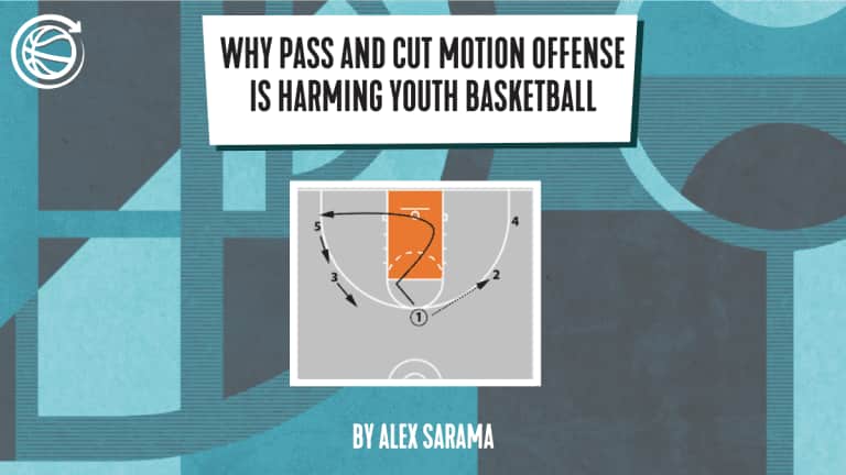
This article breaks down why pass and cut motion offense limits youth player development, and explores better ways to teach spacing, decision-making, and offensive creativity.
May 1, 2024
Alex Sarama

Approaches within the basketball industry are predominantly based upon experiential knowledge and traditions.


